I downloaded 120 KB of a 14 GB file to find the camera

The last post ended on a frustration. The train scene rendered on the Nano, real geometry in real color, but the camera would not point at the locomotive. A Gaussian scene has no canonical front, only the angles the original photos were shot from, and the file that records those angles, cameras.json, was missing from the dataset. It ships in one place, INRIA’s pretrained bundle, a single 14 GB zip.

I needed a 120 KB file out of it. Downloading 14 GB onto a 4 GB board over wifi to read a fraction of a percent was not going to happen.

A zip is a filesystem with the index at the back

The zip format saves you here. A zip is not a stream you read start to finish. It ends with a central directory, a table of every file with its name, its size, and its byte offset into the archive. Read that table and you know where any one file lives.

The server hosting the bundle accepts range requests, so a client can ask for “bytes 14,660,580,000 to the end” and get only those. The recipe follows from there. Fetch the last few kilobytes, find the central directory, fetch that, look up train/cameras.json, fetch exactly its bytes, inflate. Total pulled from a 14.66 GB archive, about 120 KB.

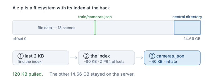
One wrinkle is size. A 14 GB archive runs past the 4 GB the original zip fields can hold, so the real offsets live in ZIP64 records, an extension bolted on for this exact case. A few extra structs to parse, and the directory gives up thirteen scenes, train/cameras.json among them. One more range request and the cameras are local, without the archive.

From a camera to a matrix

cameras.json describes each shot the plain way: where the camera stood, a 3x3 rotation for where it pointed, the focal lengths. The renderer wants two 4x4 matrices, world-to-view and the projection. The conversion is the one the reference code uses, lifted out:

# position C and rotation Rj (camera->world) from cameras.json.
Rwc = transpose(Rj)              # world->camera rotation
t   = -Rwc @ C                   # world->camera translation
# world->view is [Rwc | t]; projection comes from fx, fy and the image size.

This stays in a small Python script rather than the renderer, because the matrix algebra is four lines in Python and a chore in C++, and the renderer just reads the finished numbers.

There it is

Camera zero in the file is image 00001, the reference photo used for eyeballing all along. Rendered from it, the scene is the locomotive. Green Western Pacific 713, broadside, the hills behind, the traffic cone down front, the composition of the photograph.

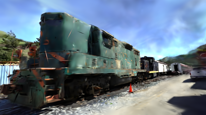
That one image settles three things at once. The point cloud and the extracted cameras share a coordinate frame, so they came from the same capture. The matrix conversion is right, because a wrong one would not land on the photo. And the anisotropic part of the renderer, the part that had only ever drawn round synthetic blobs, reconstructs a real surface correctly when fed real data and aimed from a real angle.

The honest pairing

Two numbers, and they belong to two different pictures, so neither goes under the other. The crisp render, the one that looks like the 713, keeps 150,000 splats and runs at 8 frames a second, under the target. The version that hits the target, about 17 frames a second at 480p, is pruned harder to 50,000 and is visibly softer, more watercolor than photo. Same view, same code, a sharpness-for-speed dial between them. In-band and a little blurry, or crisp and a little slow. On a 2019 board rendering a real capture, in-band and blurry takes it, stated plainly.

One footnote this owes. Matching the photograph shows the whole pipeline works end to end, but the photograph is ground truth from a camera, not the output of the reference renderer. Proving the stripped renderer agrees with the one it was carved from, pixel for pixel, means rendering the same camera with the original on a desktop and diffing. That has not run yet. So “matches the reference renderer” is a claim not yet earned, and “matches the photo it was trained on” is the one in hand.

Where this leaves it

A 2019, $99 board renders a real photogrammetry capture of a locomotive at a little under 20 frames a second, inside the target, from the angle it was shot. The renderer is a forward-only carve of the reference, patched to compile for a chip that predates half the CUDA it was written against. The speed came from profiling that corrected the obvious guesses twice, and from throwing away 93% of the scene as haze. The camera that framed it came out of a 14 GB file that stayed on the server.

Next: rendering the same camera with the stock reference renderer and diffing, pixel for pixel.

Real-time Gaussian Splatting on a $99 board

1. Compiling a 2023 CUDA renderer for a 2015 GPU
2. Gaussian Splatting on a Jetson Nano: the bottleneck wasn't the sort
3. Most of a Gaussian scene is haze: pruning a real capture onto a $99 board
4. I downloaded 120 KB of a 14 GB file to find the camera (this post)

New parts publish weekly; this list grows as each one goes live.